Hybrid Parcel Tracker - Post-Processing Analysis

1. Overview

This document describes the code structure and analysis workflow for post-processing results from Hybrid Parcel Tracker (HPT) simulations using Hybrid Parcel Tracker - Post. This tool complements Hybrid Parcel Tracker - Main by analyzing the results from particle tracking simulations. The primary goal is to analyze moisture and temperature changes along particle trajectories, identify significant events (uptake/release of moisture, warming/cooling), and visualize these phenomena through various plots and animations.

The workflow is driven by the main_analysis_workflow.py script, which utilizes a central configuration file (config.py) and calls specialized modules for data processing, analysis, plotting, and animation.

2. Code Structure

The project is organized into several Python scripts, each responsible for specific tasks:

• config.py: The master configuration file. It defines all parameters for the analysis, including file paths, event definitions, plotting extents, time ranges, and processing options.
• main_analysis_workflow.py: The central orchestrator script. It loads the configuration, manages the overall workflow by calling functions from other modules in sequence.
• data_processing.py: Handles initial data loading from augmented particle files (which can be in **CSV or NetCDF format**), identification of relevant particles, extraction of their full histories, calculation of moisture/temperature changes (Δq, ΔT for 1-hour and 6-hour windows), event classification (Uptake, Release, Warming, Cooling), calculation of mean pressure over change windows, and 1-hour pressure change (dp/dt). It culminates in creating a master DataFrame (master_df).
• plotting_2d.py: Generates various 2D static plots (aggregate maps, composite trajectory density, individual trajectories) and individual frames for 2D animations.
• plotting_3d.py: Generates 3D static trajectory plots and individual frames for 3D animations, visualizing particle paths in a 3D space (longitude, latitude, pressure).
• statistical_analysis.py: Performs a wide range of statistical analyses and generates corresponding plots. This includes vertical profiles of various quantities (overall, in-target, conditional), histograms of event magnitudes, analysis of time spent in target, release amounts in target, geographical distribution of last events, and time evolution plots.
• animations.py: Compiles the 2D and 3D frames generated by the plotting modules into animated GIFs and/or MP4 videos using the imageio library. Also handles generation of static colorbars for animations.
• tracks_analysis.py: Performs specialized trajectory analysis focusing on particles reaching a specific target region at defined times. It plots their initial positions, full trajectories, and changes in q/T along these paths.
• MoistureTracks.py: Analyzes and plots trajectories of particles that release moisture over the target area. Generates cumulative and hourly trajectory plots, aggregate moisture contribution maps, time evolution plots, and gridded moisture release data.

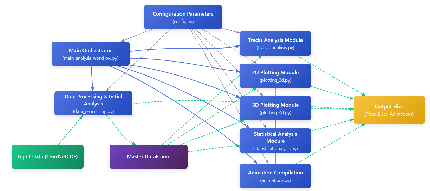Figure 1: Overall Code Structure and Data Flow Diagram - Post-Processing Analysis Workflow.

3. Configuration Parameters (config.py)

The config.py file is central to the entire workflow, allowing customization of the analysis without modifying core scripts. Below are the key configurable parameters, grouped by their purpose:

3.1. Core Simulation & Data Paths

• BASE_OUTPUT_DIR: Main directory where all analysis results will be saved.
• AUGMENTED_PARTICLE_DATA_DIR: Path to the directory containing input particle data files. These files are expected to be in **CSV or NetCDF (.nc)** format and include at least: id, time_step (or means to derive it), latitude, longitude, pressure, specific_humidity, temperature.
• ORIGINAL_PARTICLE_SIM_DIR: Optional path to raw particle simulation output, potentially used by specific legacy analysis components.

3.2. Event Definition & Initial Particle Selection

• SIMULATION_START_DATETIME: Timestamp (e.g., 'YYYY-MM-DD HH:MM:SS') corresponding to the simulation's time_step = 0.
• TARGET_LAT_CENTER: Latitude of the center of the target region.
• TARGET_LON_CENTER: Longitude of the center of the target region.
• TARGET_BOX_HALF_WIDTH_DEG: Half-width (in degrees) of the square target box. A value of 0.1 means a 0.2x0.2 degree box.
• RELEVANT_PARTICLE_TARGET_ARRIVAL_STEPS: A range or list of hours (from simulation start) during which particles arriving in the target box are considered "relevant" for the main analysis.

3.3. Detailed Analysis Configuration

• ANALYSIS_START_HOUR: Hour (0-indexed from simulation start) to begin detailed history analysis for each selected particle. For example, if particles are selected based on arrival at H48, their history will be traced back to this ANALYSIS_START_HOUR.
• EVENT_CORE_ANALYSIS_STEPS: Range or list of hours defining the primary period for analyzing specific phenomena (e.g., moisture release *within* the target *during* these hours). This can be the same as RELEVANT_PARTICLE_TARGET_ARRIVAL_STEPS or a sub-period.
• TRACK_HISTORY_WINDOW_AFTER_MAX_ARRIVAL_HOURS: Number of hours to continue tracking particle histories *after* the latest arrival step defined in RELEVANT_PARTICLE_TARGET_ARRIVAL_STEPS. This allows looking at what happens to particles *after* passing the target.
• DQ_THRESHOLD_KG_PER_KG: Threshold for significant specific humidity change (in kg/kg) over CHANGE_WINDOW_HOURS to define moisture uptake/release events.
• DT_THRESHOLD_KELVIN: Threshold for significant temperature change (in Kelvin) over CHANGE_WINDOW_HOURS to define warming/cooling events.
• CHANGE_WINDOW_HOURS: Time window (in hours) used for calculating Δq and ΔT for event definition (typically 6 hours). 1-hour changes are also calculated separately.

3.4. Plotting & Animation Configuration

• FIXED_PLOT_EXTENT_2D: Optional tuple (lon_min, lon_max, lat_min, lat_max) for 2D plots. If None, extent is dynamic.
• FIXED_PLOT_LONLAT_EXTENT_3D: Optional tuple (lon_min, lon_max, lat_min, lat_max) for the longitude/latitude extent of 3D plots. If None, extent is dynamic.
• FIXED_PLOT_PRESSURE_EXTENT_3D: Optional tuple (p_min_hPa, p_max_hPa) for the pressure extent of 3D plots. If None, extent is dynamic.
• DEFAULT_PLOT_VIEW_ANGLE_3D: Tuple (elevation, azimuth) for the default camera view in 3D plots.
• DEFAULT_PLOT_BUFFER_DEG: Buffer (in degrees) added to dynamic plot extents if fixed extents are not used.
• ANIMATION_FRAME_START_HOUR: Starting hour for generating animation frames.
• ANIMATION_FRAME_END_HOUR: Ending hour (inclusive) for generating animation frames.
• ANIMATION_FPS: Frames per second for output animations.
• ANIMATION_DPI: Dots per inch for saved animation frames.
• MAX_INDIVIDUAL_TRAJECTORIES_TO_PLOT: Maximum number of individual particle trajectories to plot for detailed static plots. If None, attempts to plot all relevant ones.
• TIME_EVOLUTION_FOCUS_STEPS: List of specific hours for which to generate focused time-evolution plots (particles arriving at these hours).
• AGGREGATE_MAP_GRID_RESOLUTION_DEG: Grid resolution (in degrees) for 2D aggregate heatmap plots.
• CMAP_SPECIFIC_HUMIDITY, CMAP_TEMPERATURE, etc.: Names of Matplotlib colormaps used for various plots.
• TARGET_AREA_PLOT_COLOR: Color used to display the target area in plots.
• AGGREGATE_COLOR_PERCENTILES: Tuple (min_percentile, max_percentile) for robust color scaling in aggregate maps (e.g., sum of dq/dt).
• PRESSURE_BINS_CATEGORICAL: NumPy array defining pressure bins (hPa) for categorical coloring (e.g., in Tracks analysis).
• VERTICAL_PROFILE_PRESSURE_BINS: NumPy array defining pressure bins (hPa) for finer vertical profile analyses.
• DATETIME_PLOT_FORMAT: String format for displaying datetimes in plot titles and labels (e.g., "%Y-%m-%d %H:%M").

3.5. Tracks Analysis Specific Settings

• TRACKS_PARTICLE_SOURCE_FOLDER: Typically same as AUGMENTED_PARTICLE_DATA_DIR for the `run_tracks_analysis_from_master` workflow.
• TRACKS_TARGET_STEPS: List or range of hours for which the tracks analysis specifically identifies particles arriving in the target. Often same as RELEVANT_PARTICLE_TARGET_ARRIVAL_STEPS.
• TRACKS_PLOT_EXTENT_2D: Optional fixed 2D plotting extent (lon_min, lon_max, lat_min, lat_max) specifically for plots generated by `tracks_analysis.py`. If None, extent is dynamic.
• (Other parameters like TARGET_LAT_CENTER, ANALYSIS_START_HOUR, TRACK_HISTORY_WINDOW_AFTER_MAX_ARRIVAL_HOURS are also used by Tracks Analysis).

3.6. Parallel Processing

• NUM_WORKERS: Number of worker processes to use for parallelizable tasks. Defaults to cpu_count() - 1.

3.7. Output Subdirectory Definitions

These parameters define the names of subdirectories within BASE_OUTPUT_DIR where different types of outputs are stored. Examples:

• DATA_PROCESSING_OUTPUT_DIR (derived, e.g., BASE_OUTPUT_DIR / "1_processed_data")
• RELEVANT_IDS_FILE (path to file)
• FILTERED_HOURLY_DATA_DIR (path to directory)
• ANALYZED_PARTICLE_HISTORIES_DIR (path to directory)
• PLOTS_OUTPUT_DIR (derived, e.g., BASE_OUTPUT_DIR / "2_plots_and_animations")
• TRACKS_OUTPUT_DIR (path to directory)
• INDIVIDUAL_TRAJ_PLOTS_SUBDIR (name of subdirectory)
• AGGREGATE_MAPS_MOISTURE_SUBDIR (name of subdirectory)
• ... and other subdirectory names for animations, statistical plots, etc.

Note: Some parameters like MAX_HISTORY_TRACKING_HOUR are derived by the main script based on other configurations and should not be set manually.

4. Main Workflow (main_analysis_workflow.py)

The main script orchestrates the entire post-processing pipeline. The typical flow is as follows:

Figure 2: Flowchart of main_analysis_workflow.py - Main Analysis Workflow Stages.

4.1. Setup

• Initializes logging using setup_logging.py (not explicitly shown in `main_analysis_workflow.py` but good practice).
• Calls create_output_directories() to establish the necessary folder structure based on config.py settings.
• Calculates derived configuration values, such as MAX_HISTORY_TRACKING_HOUR.

4.2. Stage 1: Identify Relevant Particle IDs

• Calls data_processing.identify_target_particles_from_augmented_data().
• Purpose: To find unique particle IDs that pass through the defined TARGET_LAT_CENTER, TARGET_LON_CENTER, TARGET_BOX_HALF_WIDTH_DEG during the hours specified in RELEVANT_PARTICLE_TARGET_ARRIVAL_STEPS.
• Input: Augmented particle data CSVs from AUGMENTED_PARTICLE_DATA_DIR.
• Output: A list of relevant particle IDs, saved to RELEVANT_IDS_FILE.

4.3. Stage 2: Extract Full Histories for Relevant Particles

• Calls data_processing.extract_particle_histories().
• Purpose: To gather the complete time-series data for the identified relevant particles.
• Input: The list of relevant IDs, augmented particle data CSVs.
• Parameters: Histories are extracted from ANALYSIS_START_HOUR up to the calculated MAX_HISTORY_TRACKING_HOUR.
• Output: Filtered hourly CSV files (containing only relevant particles) in FILTERED_HOURLY_DATA_DIR.

4.4. Stage 3: Analyze Histories for Moisture & Temperature Changes

• Calls data_processing.analyze_all_particle_histories_detailed().
• Purpose: To calculate changes in specific humidity (Δq) and temperature (ΔT), identify atmospheric events, and compute related pressure metrics for each relevant particle.
• Input: Filtered hourly data from Stage 2.
• Parameters: Uses DQ_THRESHOLD_KG_PER_KG, DT_THRESHOLD_KELVIN, and CHANGE_WINDOW_HOURS (for 6-hour changes) and a fixed 1-hour window for 1-hour changes.
• Output: CSV files for each analyzed particle (e.g., particle_{id}_analyzed_history.csv) in ANALYZED_PARTICLE_HISTORIES_DIR, containing original data plus new columns for Δq, ΔT (1hr & 6hr), event types, mean pressures, and dp/dt.

4.5. Stage 4: Load Master DataFrame for Plotting & Further Analysis

• Calls data_processing.load_master_analyzed_df().
• Purpose: To consolidate all individual analyzed particle histories into a single, comprehensive Pandas DataFrame.
• Input: Analyzed particle history CSVs from Stage 3.
• Output: The master_df DataFrame, which is then used by subsequent analysis and plotting stages.

4.6. Stage 5: Tracks Analysis

• Calls tracks_analysis.run_tracks_analysis_from_master().
• Purpose: To perform a specialized analysis focusing on particles arriving at the target region during specific steps (TRACKS_TARGET_STEPS).
• Input: The master_df and configuration object.
• Output: CSV files with initial/final states of target-reaching particles, and various plots (initial positions, trajectory maps, q/T change along tracks) saved in TRACKS_OUTPUT_DIR.

4.7. Stage 6: Generate Plots and Animations

This stage involves calls to multiple functions from different modules, using the master_df and config_obj.

• 2D Aggregate Maps (plotting_2d.plot_aggregate_map_generic):
  • Net change maps for moisture (dq/dt) and temperature (dT/dt).
  • Frequency maps for Uptake, Release, Warming, and Cooling events.
• Composite Trajectory Density Plot (plotting_2d.plot_composite_trajectory_density): Visualizes all relevant particle trajectories with event locations.
• Statistical Distributions & Profiles (various functions in statistical_analysis.py):
  • Vertical profiles of average dq/dt and dT/dt.
  • Histograms of event magnitudes.
  • Geographical distribution of last significant events before target arrival.
  • Analysis of time spent in target and release amounts within the target.
  • Vertical profiles of q, T, dq/dt, dT/dt specifically within the target region.
  • Vertical profiles of 1-hr and 6-hr changes vs. mean pressure over the change window.
  • Conditional vertical profiles in the target (e.g., dq/dt vs. pressure, conditioned by ascent/descent).
  • Profiles of net q/T change during target transit.
  • Scatter plots of current q/T vs. lagged q/T within the target.
• Time Evolution Plots (statistical_analysis.plot_time_evolution_multi_step, statistical_analysis.plot_time_evolution_full_event):
  • Mean q/T and event counts over time, aligned by specific arrival hours or first arrival in target.
• Individual Trajectory Plots:
  • plotting_2d.plot_selected_individual_2d_trajectories: 2D plots for selected particles.
  • plotting_3d.plot_selected_individual_3d_trajectories: 3D plots for selected particles.
• Animations (animations.create_all_animations):
  • Generates 2D and 3D hourly snapshot animations (GIF, MP4) and static colorbars.

4.8. Stage 7: Moisture Tracks Analysis

• Calls MoistureTracks.run_moisture_tracks_analysis(master_df, config_obj).
• Purpose: To identify particles releasing moisture in the target area, analyze their trajectories and spatial contributions.
• Output: Trajectory plots (hourly, cumulative), moisture contribution maps, time evolution plots, Excel files with detailed data, all saved in MOISTURE_TRACKS_OUTPUT_DIR.

5. Detailed Analyses & Methodologies

5.1. Data Processing (data_processing.py)

This module is responsible for preparing the data for all subsequent analyses.

5.1.1. Identifying Target Particles (identify_target_particles_from_augmented_data)

This function reads particle data files (expected to be hourly CSVs or NetCDFs) from the AUGMENTED_PARTICLE_DATA_DIR.

• Purpose: Selects particles that enter a defined target region during specified time steps.
• Method: Iterates through hourly augmented data files for each hour in RELEVANT_PARTICLE_TARGET_ARRIVAL_STEPS. For each file, it checks which particles fall within the geographical box defined by TARGET_LAT_CENTER, TARGET_LON_CENTER, and TARGET_BOX_HALF_WIDTH_DEG. Unique IDs are collected.
• Output: A CSV file (RELEVANT_IDS_FILE) listing unique particle IDs.

5.1.2. Extracting Particle Histories (extract_particle_histories)

• Purpose: Gathers the full trajectory data for the previously identified relevant particles over a specified analysis period. This involves reading the original augmented data files (CSVs or NetCDFs) again.
• Input: The list of relevant IDs, augmented particle data files from AUGMENTED_PARTICLE_DATA_DIR.
• Method: For each hour from ANALYSIS_START_HOUR to MAX_HISTORY_TRACKING_HOUR, it reads the corresponding augmented data file, filters it for the relevant particle IDs, and saves the filtered data to a new hourly file in FILTERED_HOURLY_DATA_DIR. The time_step column is ensured.

5.1.3. Detailed History Analysis (analyze_all_particle_histories_detailed via _analyze_single_particle_history_worker)

• Purpose: Calculates changes in moisture and temperature, classifies events, and computes pressure-related metrics for each particle's history.
• Methodology (per particle):
  1. Concatenates all hourly filtered data for the particle.
  2. Moisture/Temperature Change (Δq, ΔT):

     Calculated for two windows:

     • Over CHANGE_WINDOW_HOURS (typically 6 hours):
       Δq_6hr(t) = q(t) - q(t - CHANGE_WINDOW_HOURS)
       ΔT_6hr(t) = T(t) - T(t - CHANGE_WINDOW_HOURS)
       These are stored as dq_dt_6hr and dT_dt_6hr.
     • Over 1 hour:
       Δq_1hr(t) = q(t) - q(t - 1 hour)
       ΔT_1hr(t) = T(t) - T(t - 1 hour)
       These are stored as dq_dt_1hr and dT_dt_1hr.

  3. Event Identification (based on 6-hour changes):
     • Moisture Uptake: if Δq_6hr ≥ DQ_THRESHOLD_KG_PER_KG (column moisture_event_type)
     • Moisture Release: if Δq_6hr ≤ -DQ_THRESHOLD_KG_PER_KG
     • Warming: if ΔT_6hr ≥ DT_THRESHOLD_KELVIN (column temp_event_type)
     • Cooling: if ΔT_6hr ≤ -DT_THRESHOLD_KELVIN
     • Neutral: Otherwise.
  4. Pressure Metrics:
     • Mean Pressure over Window:
       P_mean,6hr(t) = (P(t) + P(t - CHANGE_WINDOW_HOURS)) / 2 (column mean_pressure_6hr_window)
       P_mean,1hr(t) = (P(t) + P(t - 1 hour)) / 2 (column mean_pressure_1hr_window)
     • 1-hour Pressure Change (Vertical Motion Proxy):
       ΔP_1hr(t) = P(t) - P(t - 1 hour) (column dp_dt_1hr; negative implies ascent)
• Output: Individual CSV files per particle in ANALYZED_PARTICLE_HISTORIES_DIR, containing all original and newly computed columns.

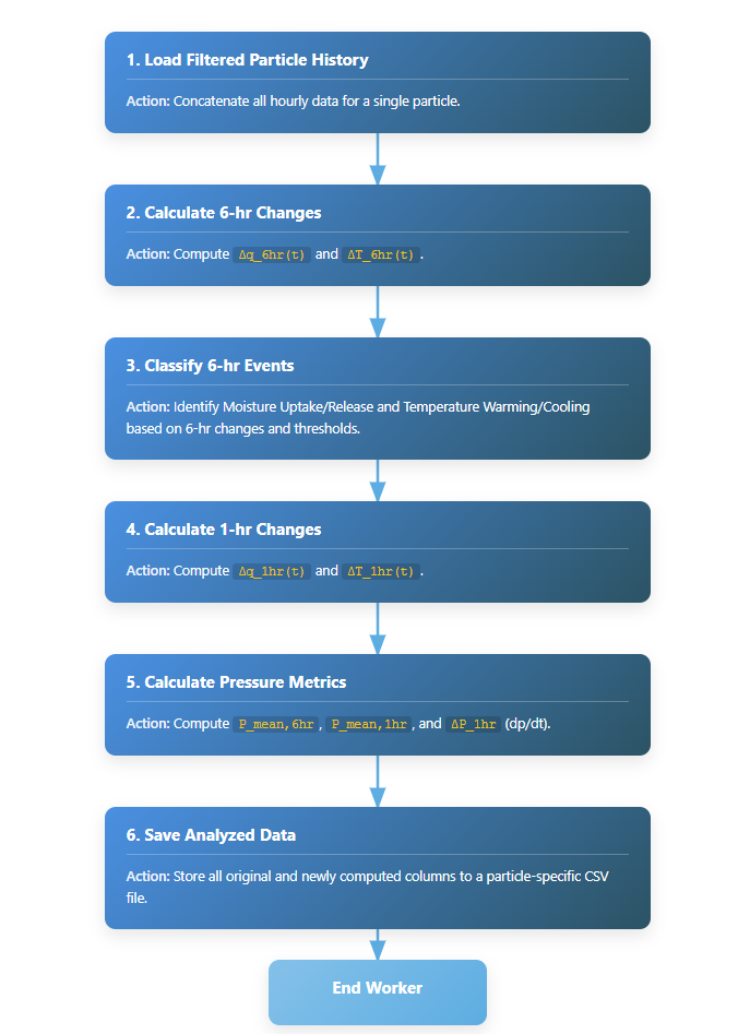Figure 3: Flowchart of Detailed History Analysis per particle (Δq, ΔT calculation) - Single Particle History Analysis Workflow.

5.1.4. Loading Master DataFrame (load_master_analyzed_df)

• Purpose: Consolidates all individual analyzed particle data into a single DataFrame.
• Method: Reads all particle_{id}_analyzed_history.csv files from ANALYZED_PARTICLE_HISTORIES_DIR (optionally filtered by relevant_ids_list) and concatenates them. Ensures correct data types and sorts by particle ID and time step.
• Output: The master_df.

5.2. Tracks Analysis (tracks_analysis.py)

This module performs analysis focused on particles that interact with a predefined target area during specific time steps, similar to the "Tracks21" methodology. It uses the master_df as its primary input.

5.2.1. Main Function: run_tracks_analysis_from_master (calls process_track_step_from_master)

This function orchestrates the tracks analysis for each target step specified in TRACKS_TARGET_STEPS.

• Purpose: For each hour in TRACKS_TARGET_STEPS, identify particles within the target, trace their histories, and generate specific plots and data.
• Key Configuration Parameters:
  • TRACKS_TARGET_STEPS: Hours for target arrival analysis.
  • TARGET_LAT_CENTER, TARGET_LON_CENTER, TARGET_BOX_HALF_WIDTH_DEG: Target area definition.
  • ANALYSIS_START_HOUR: Reference hour for initial positions and start of trajectory tracing.
  • TRACKS_PLOT_EXTENT_2D: Optional fixed extent for 2D track plots.
  • PRESSURE_BINS_CATEGORICAL, CMAP_PRESSURE: For pressure-colored plots.
  • TRACK_HISTORY_WINDOW_AFTER_MAX_ARRIVAL_HOURS: Duration to track q/T changes *after* target arrival.
• Methodology & Outputs (per target step hour, via process_track_step_from_master):
  1. Particle Identification: Selects particles from master_df that are within the target box at the current target_step_hour.
  2. Initial and Final States CSV: For these particles, extracts their state (position, pressure, q, T) at ANALYSIS_START_HOUR (initial) and at target_step_hour (final). Saves to a CSV file in TRACKS_OUTPUT_DIR/data_from_master/.
  3. Initial Position Plots: Generates a 2D map showing initial positions (ANALYSIS_START_HOUR) of particles arriving at the target. Points are colored by initial pressure. Saved in TRACKS_OUTPUT_DIR/plots_from_master/.
  4. Trajectory Plots (Map View): Generates a 2D map showing full trajectories from ANALYSIS_START_HOUR to target_step_hour. Start/end points marked and colored by pressure. Saved in TRACKS_OUTPUT_DIR/plots_from_master/.
  5. Property Change Along Trajectory Plots: For each selected particle, plots time series of its specific humidity (q, in g/kg) and temperature (T, in K). The time axis uses actual datetimes and covers from ANALYSIS_START_HOUR up to target_step_hour + TRACK_HISTORY_WINDOW_AFTER_MAX_ARRIVAL_HOURS. The target arrival time is marked. Saved in TRACKS_OUTPUT_DIR/plots_from_master/change_along_trajectory/.

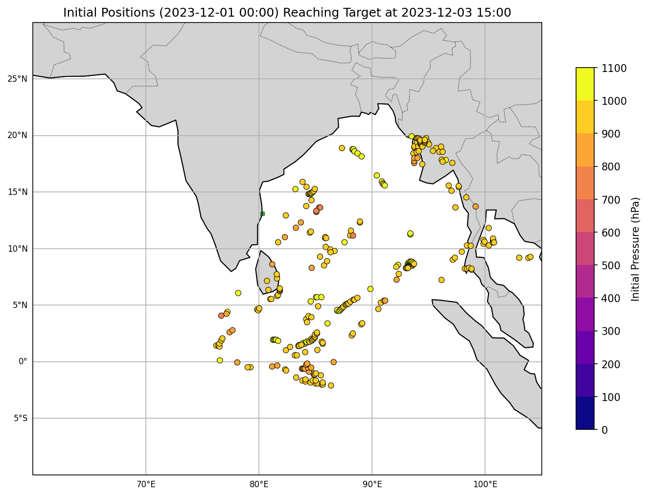Figure 4: Example Plot of Initial Positions (Tracks Analysis).

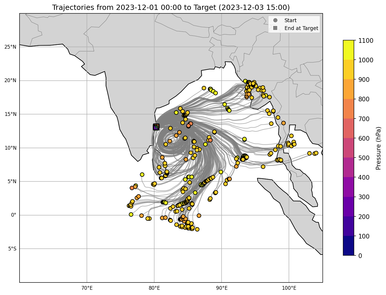Figure 5: Example Trajectory Map for Target-Reaching Particles (Tracks Analysis).

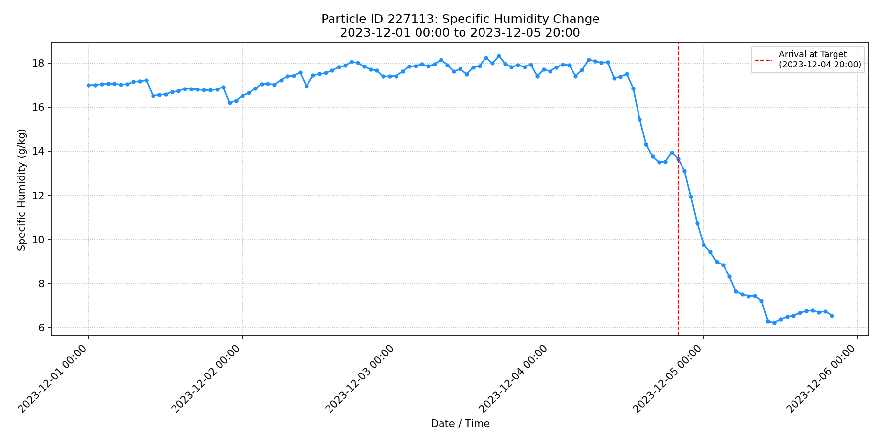Figure 6: Example Plot of Specific Humidity Change Along a Particle Track (Tracks Analysis).

5.3. 2D Plotting (plotting_2d.py)

This module generates various 2D static visualizations and frames for 2D animations.

5.3.1. Aggregate Maps (plot_aggregate_map_generic)

These plots show spatial distributions of event frequencies or net changes across all relevant particle trajectories.

• Purpose: To show spatial distributions of event frequencies or net changes.
• Methodology: Uses scipy.stats.binned_statistic_2d to grid particle event data.
  • Frequency Maps: Counts occurrences of "Uptake", "Release", "Warming", or "Cooling" events per grid cell.
  • Net Change Maps: Sums dq_dt (converted to g/kg) or dT_dt (K) per grid cell for "AllEvents" (non-neutral).
• Key Configuration: FIXED_PLOT_EXTENT_2D, AGGREGATE_MAP_GRID_RESOLUTION_DEG, various CMAP_* settings, TARGET_AREA_PLOT_COLOR.
• Output: PNG images in PLOTS_OUTPUT_DIR/aggregate_maps/.

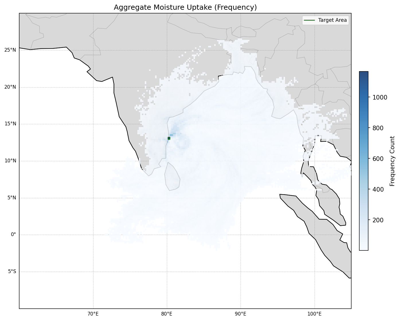Figure 7: Example Aggregate Moisture Uptake Frequency Map.

5.3.2. Composite Trajectory Density Plot (plot_composite_trajectory_density)

• Purpose: Visualizes the path of all relevant particle trajectories on a single map, with event locations overlaid.
• Methodology: Plots each particle's path with low alpha. Scatter plots mark locations of "Uptake" (blue) and "Release" (red) events. The target area is also shown.
• Output: PNG image in PLOTS_OUTPUT_DIR/aggregate_maps/.

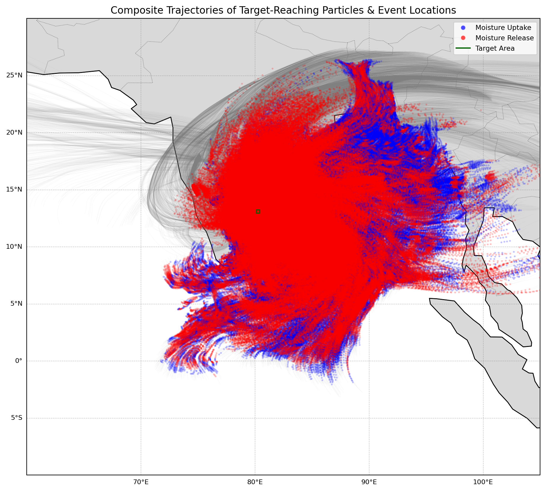Figure 8: Example Composite Trajectory Density Plot.

5.3.3. Individual 2D Trajectories (plot_selected_individual_2d_trajectories via _plot_individual_2d_trajectory_detailed_worker)

• Purpose: Detailed 2D visualization of individual particle paths for a selected subset of particles.
• Methodology: For a selection of particles (up to MAX_INDIVIDUAL_TRAJECTORIES_TO_PLOT), plots the 2D path (longitude vs. latitude). Trajectories are colored by pressure using CMAP_PRESSURE and PRESSURE_BINS_CATEGORICAL. Significant moisture/temperature events (Uptake, Release, Warming, Cooling) are marked along the path. Start/end points and target area are shown.
• Output: PNG images in PLOTS_OUTPUT_DIR/individual_trajectories/Moisture (or /Temperature).

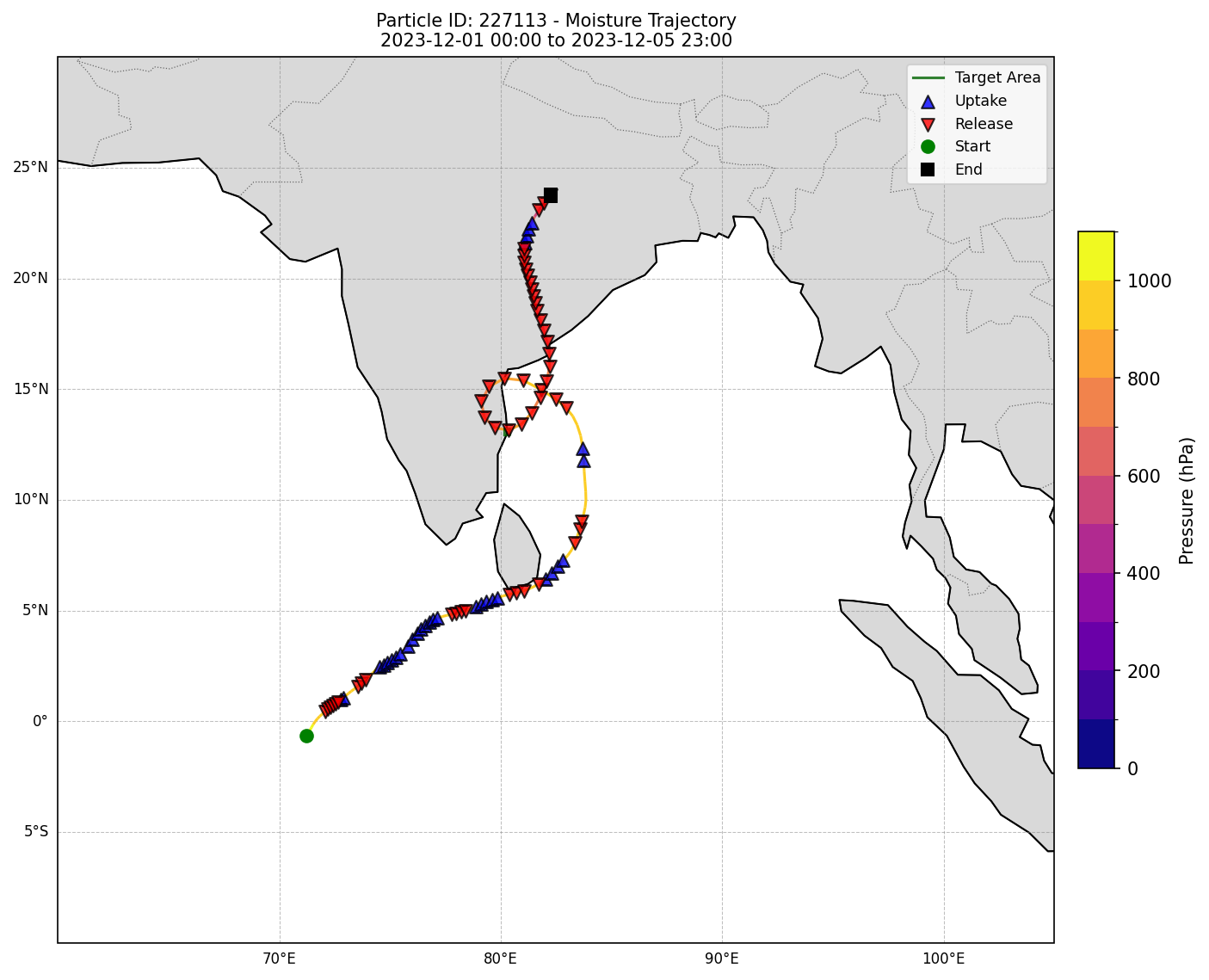Figure 9: Example Individual 2D Particle Trajectory with Events.

5.4. 3D Plotting (plotting_3d.py)

This module generates 3D static visualizations and frames for 3D animations.

5.4.1. Individual 3D Trajectories (plot_selected_individual_3d_trajectories via _plot_one_static_3d_traj)

These plots provide a 3D view of selected particle paths, including pressure changes.

• Purpose: Detailed 3D visualization of individual particle paths.
• Methodology: For selected particles, plots the 3D path (longitude, latitude, pressure). Trajectories are colored by a scalar variable (specific humidity or temperature). Event locations (Uptake/Release or Warming/Cooling), the 3D target volume, coastlines, and a floor representing the plot boundary are visualized.
• Key Configuration: FIXED_PLOT_LONLAT_EXTENT_3D, FIXED_PLOT_PRESSURE_EXTENT_3D, DEFAULT_PLOT_VIEW_ANGLE_3D, CMAP_SPECIFIC_HUMIDITY, CMAP_TEMPERATURE.
• Output: PNG images in PLOTS_OUTPUT_DIR/individual_trajectories/3D/.

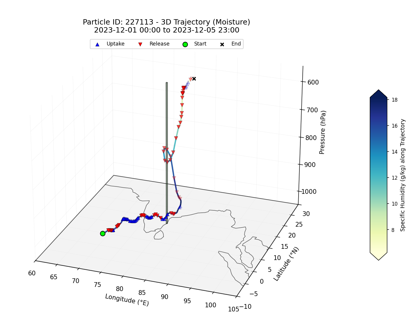Figure 10: Example Individual 3D Particle Trajectory.

5.5. Statistical Analysis (statistical_analysis.py)

This module provides a suite of functions for statistical characterization of particle behavior and atmospheric events.

5.5.1. Vertical Profile of Changes (plot_vertical_profile_change)

• Purpose: Shows average Δq or ΔT versus pressure for different event types (Uptake/Release, Warming/Cooling) across all trajectories.
• Methodology: Filters master_df for specific events. Bins data by pressure (VERTICAL_PROFILE_PRESSURE_BINS) and calculates the mean of dq_dt (g/kg per X hrs) or dT_dt (K per X hrs) in each bin.
• Output: Line plots saved in PLOTS_OUTPUT_DIR/statistical_distributions/.

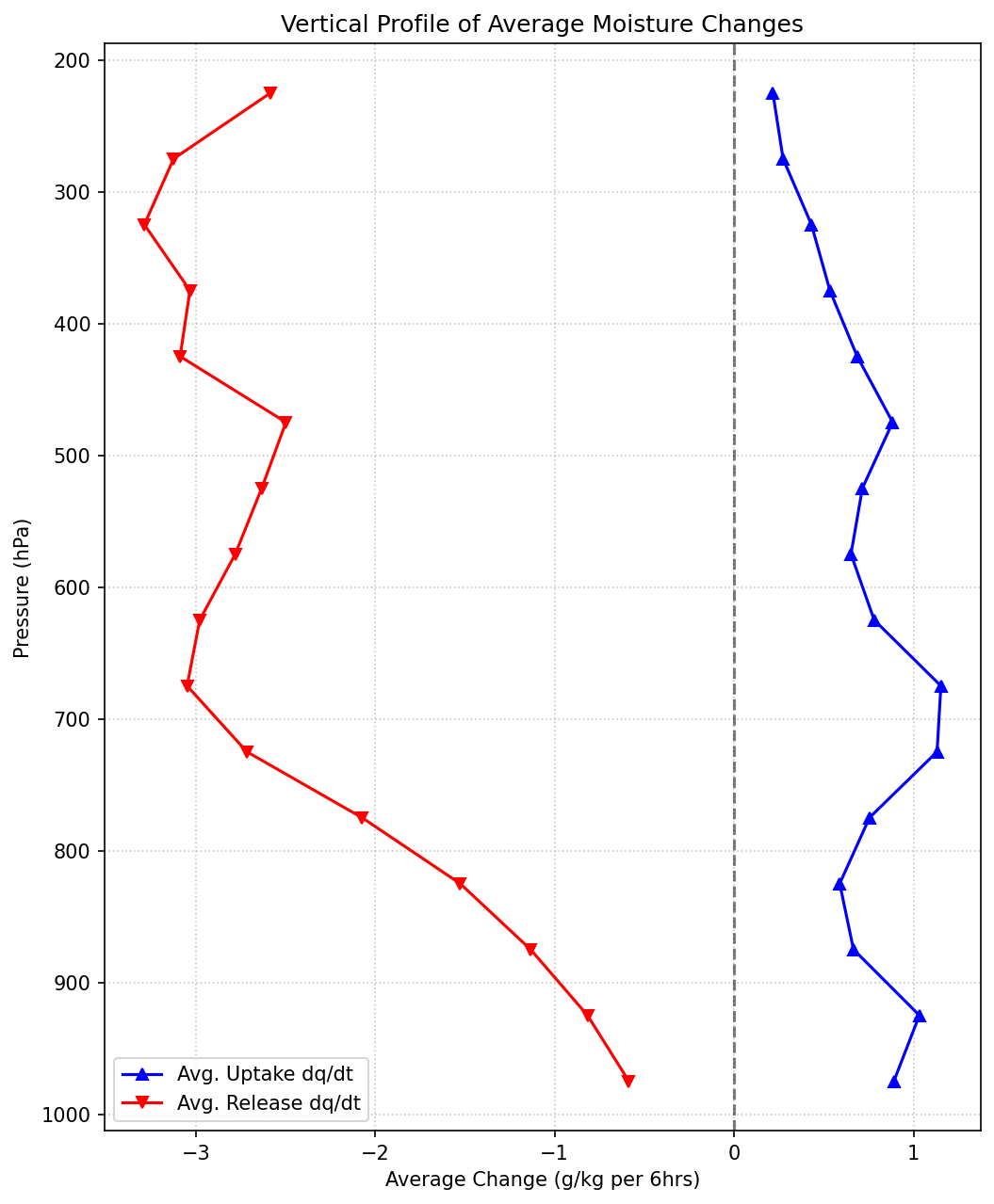Figure 11: Example Vertical Profile of Average Moisture Change.

5.5.2. Histogram of Event Magnitudes (plot_histogram_event_magnitudes)

These histograms show the distribution of the strength of significant uptake/release events.

• Purpose: Displays the distribution of the magnitudes of Δq or ΔT for identified events.
• Methodology: Filters for Uptake/Release (or Warming/Cooling) events and plots histograms of their dq_dt or dT_dt values.
• Output: Histograms saved in PLOTS_OUTPUT_DIR/statistical_distributions/.

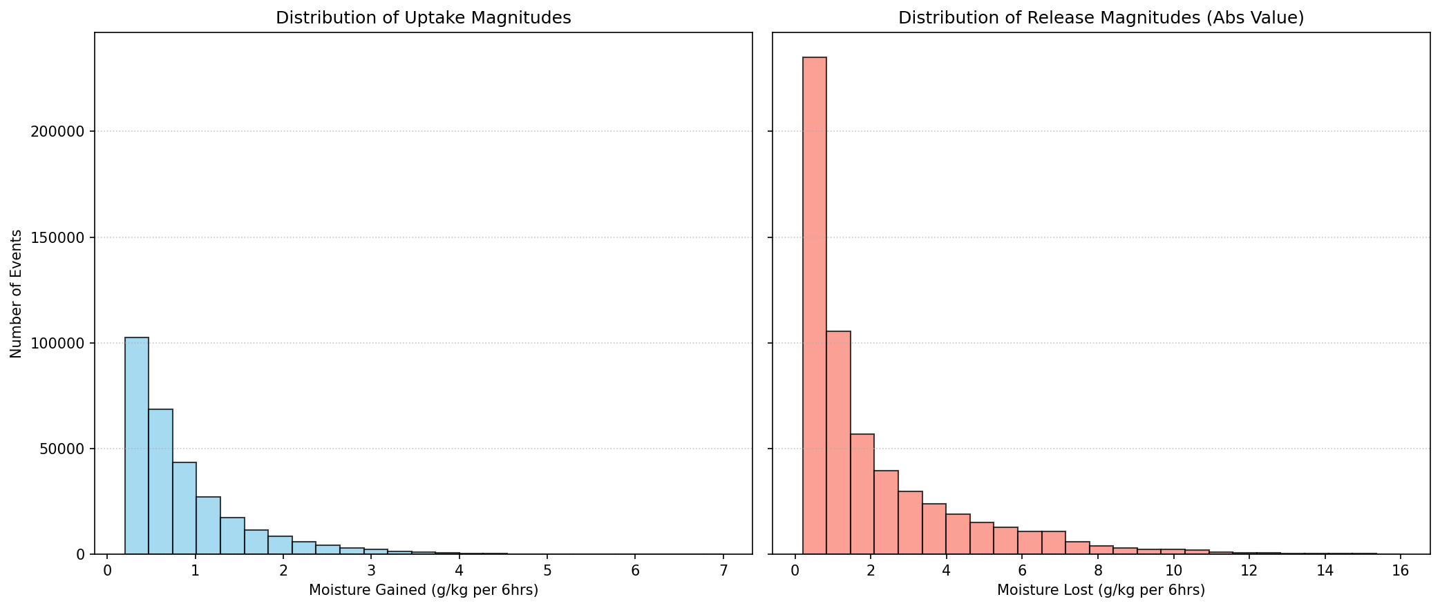Figure 12: Example Histogram of Moisture Uptake Magnitudes.

5.5.3. Geographical Distribution of Last Event Points (plot_last_event_points)

This map helps identify potential source regions for particles experiencing significant events just before reaching the target.

• Purpose: Maps the locations where particles experienced their last significant "Uptake" (or "Warming") event *before* first arriving in the target area during EVENT_CORE_ANALYSIS_STEPS.
• Methodology: For each relevant particle, finds its first arrival time in the target during the core event period. Then, searches its history *before* this arrival for the last occurrence of the specified event (e.g., "Uptake"). Plots these locations on a map, colored by pressure.
• Output: Map plots saved in PLOTS_OUTPUT_DIR/aggregate_maps/.

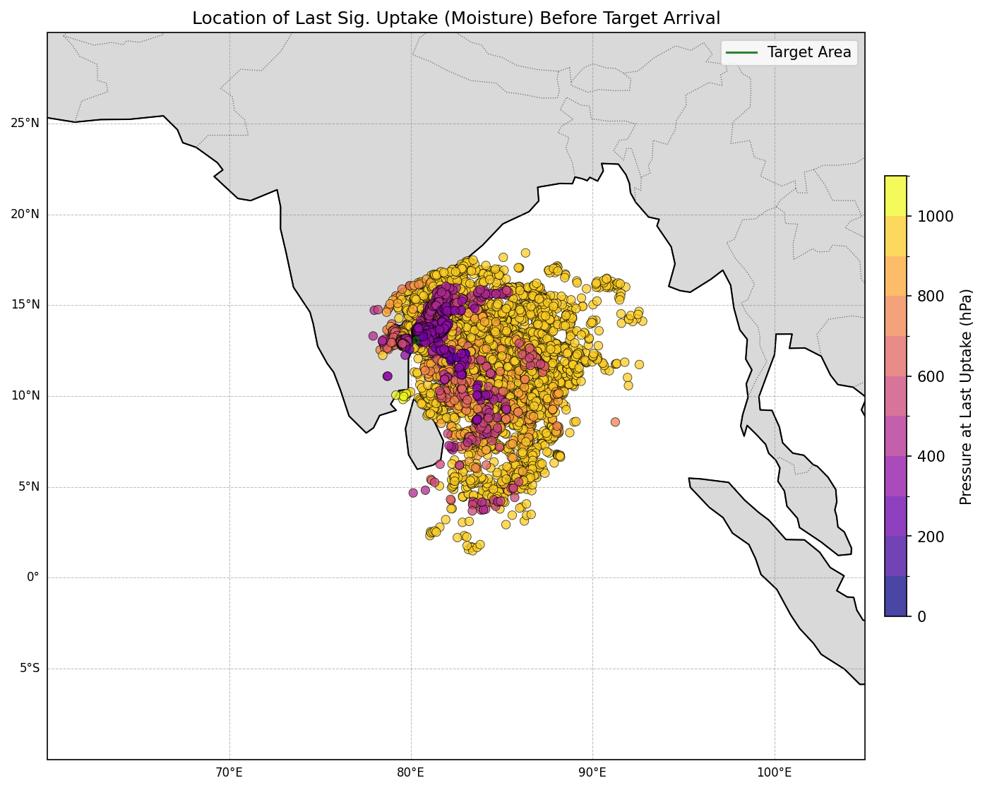Figure 13: Example Map of Last Uptake Points.

5.5.4. Time Spent in Target (analyze_and_plot_time_in_target)

Quantifies the duration particles spend within the defined target region during the core event period.

• Purpose: Quantifies how long relevant particles spend within the target region during EVENT_CORE_ANALYSIS_STEPS.
• Methodology: Filters master_df for time steps where particles are inside the target box during the core event. Counts the number of such hourly records per particle.
• Output: A CSV file (time_spent_in_target.csv) and a histogram showing the distribution of time spent in target, saved in PLOTS_OUTPUT_DIR/target_area_analysis/.

5.5.5. Release/Cooling Amount in Target (analyze_and_plot_release_in_target)

• Purpose: Quantifies the total amount of moisture (or heat) released (or lost) by particles *while they are inside the target region* during EVENT_CORE_ANALYSIS_STEPS.
• Methodology: Filters for "Release" (or "Cooling") events occurring within the target box during core event steps. Sums the dq_dt (or dT_dt) values for each particle during these events. Note that dq_dt/dT_dt are rates over CHANGE_WINDOW_HOURS.
• Output: A CSV file (e.g., total_moisture_release_in_target.csv) and a histogram of these total release amounts, saved in PLOTS_OUTPUT_DIR/target_area_analysis/.

5.5.6. Vertical Profile of Variables in Target (plot_vertical_profile_in_target)

• Purpose: Shows the average of a specified variable (e.g., q, T, dq/dt_1hr, dT/dt_1hr) versus pressure, specifically for particle segments *within the target region* during EVENT_CORE_ANALYSIS_STEPS.
• Methodology: Filters master_df for data points inside the target box during core event steps. Bins these points by their current pressure and calculates the mean of the specified value_col_to_avg in each pressure bin.
• Output: Line plots saved in PLOTS_OUTPUT_DIR/target_area_analysis/.

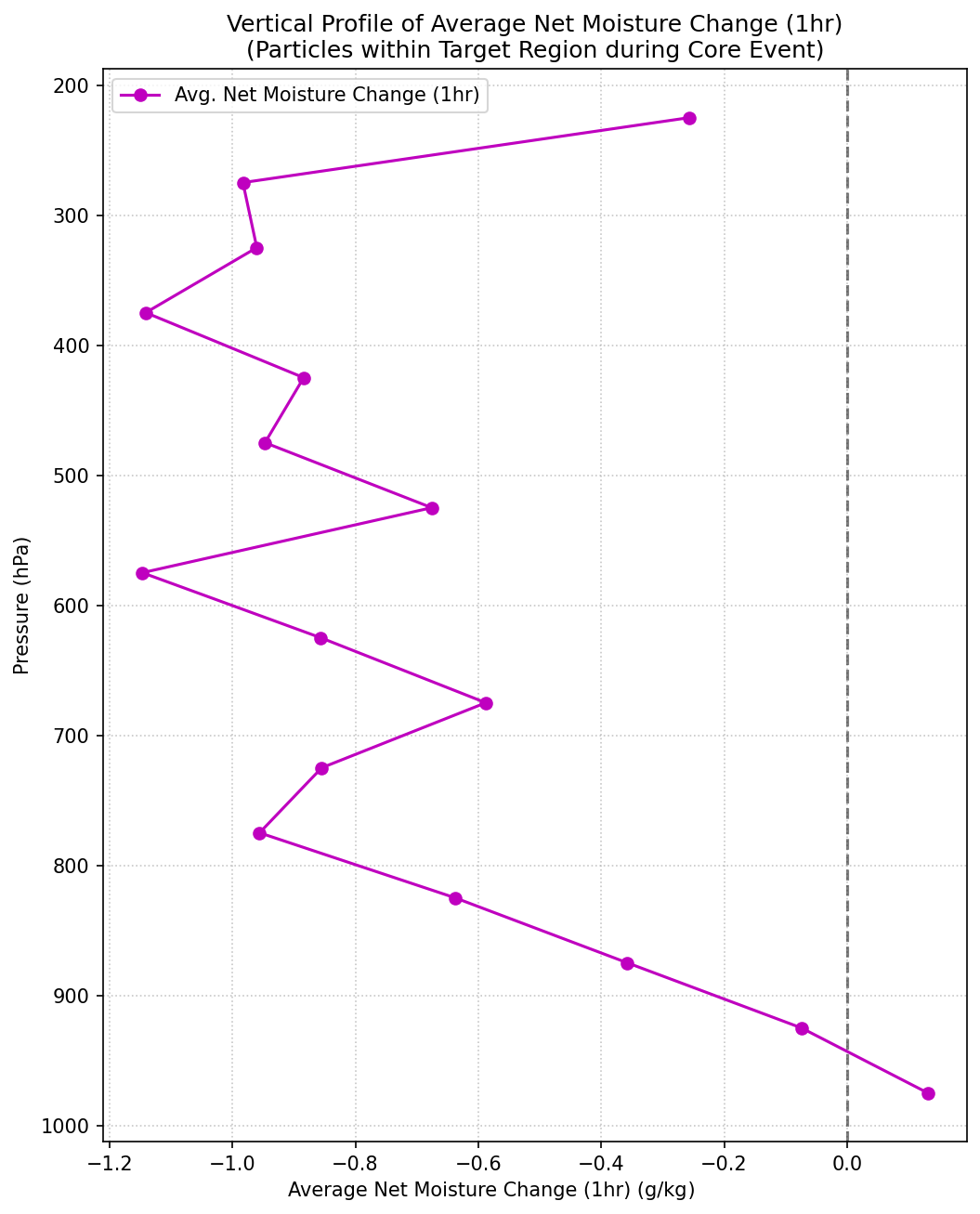Figure 14: Example Vertical Profile of Average Specific Humidity in Target.

5.5.7. Vertical Profile of Change vs. Mean Pressure (plot_vertical_profile_change_vs_mean_pressure)

• Purpose: Investigates how 1-hour or 6-hour changes in q/T relate to the average pressure level over which the change occurred, for all trajectory points.
• Methodology: Uses dq_dt_1hr/dT_dt_1hr (or dq_dt_6hr/dT_dt_6hr) and the corresponding mean_pressure_1hr_window (or mean_pressure_6hr_window). Bins by mean pressure and plots the average change in q/T for "Uptake"/"Warming" and "Release"/"Cooling" type events (event type based on 6hr change).
• Output: Line plots saved in subdirectories of PLOTS_OUTPUT_DIR/statistical_distributions/.

5.5.8. Conditional Vertical Profiles in Target (plot_conditional_vertical_profiles_in_target)

• Purpose: Examines how 1-hour or 6-hour changes in q/T within the target region vary with pressure, conditioned on whether particles are ascending, descending, or in near-neutral vertical motion.
• Methodology: Filters for data points within the target during core event steps. Uses dp_dt_1hr to classify vertical motion (ascent: dp_dt_1hr < -threshold, descent: dp_dt_1hr > threshold). For each category, bins by current pressure and plots the average dq_dt or dT_dt (for the specified time_window_hrs).
• Output: Line plots saved in PLOTS_OUTPUT_DIR/target_area_analysis/.

5.5.9. Profile of Net Change During Target Transit (plot_in_target_change_profile)

• Purpose: Calculates the net change in q/T for individual particles from the moment they enter the target box to when they exit it (during EVENT_CORE_ANALYSIS_STEPS), and plots this net change against their average pressure while in the target.
• Methodology: For each particle, identifies continuous segments where it's inside the target. Calculates Δq = q_exit - q_entry and ΔT = T_exit - T_entry for each segment. Also calculates the average pressure during that transit. Bins these Δq/ΔT values by average pressure and plots the mean.
• Output: A CSV file of transit details and line plots saved in PLOTS_OUTPUT_DIR/target_area_analysis/.

5.5.10. Current vs. Lagged Value Scatter Plot in Target (plot_q_vs_q_lagged_in_target)

• Purpose: Visualizes the relationship between the current q (or T) and its value 1 or 6 hours prior, for particle segments within the target region. Points are colored by the change over that window.
• Methodology: Filters for data points within the target during core event steps. Creates a scatter plot of specific_humidity (or temperature) against its lagged counterpart (q_lagged_1hr/6hr or T_lagged_1hr/6hr). Points are colored by dq_dt_1hr/6hr (or dT_dt_1hr/6hr). A 1:1 line indicates no change.
• Output: Scatter plots saved in PLOTS_OUTPUT_DIR/target_area_analysis/.

5.5.11. Time Evolution Plots (plot_time_evolution_multi_step, plot_time_evolution_full_event)

• Purpose: To show the average evolution of q/T and the frequency of associated events for ensembles of particles, aligned by their arrival time at the target.
• plot_time_evolution_multi_step:
  • Focuses on cohorts of particles arriving at the target at specific hours defined in TIME_EVOLUTION_FOCUS_STEPS.
  • For each cohort, aligns their histories relative to their arrival time at that focus step. The x-axis is absolute datetime.
  • Plots mean q/T (with std dev shading) and counts of Uptake/Release (or Warming/Cooling) events over time.
• plot_time_evolution_full_event:
  • Considers all relevant particles that arrive in the target at any point during EVENT_CORE_ANALYSIS_STEPS.
  • Aligns their histories relative to their *first* arrival time in the target. The x-axis is hours relative to this first arrival.
  • Plots mean q/T (with std dev shading) and event counts.
• Output: Time series plots saved in PLOTS_OUTPUT_DIR/time_evolution/.

5.5.12. Vertical Profile of Change vs. Mean Pressure (plot_vertical_profile_change_vs_mean_pressure)

• Purpose: Investigates how 1-hour or 6-hour changes in q/T relate to the average pressure level over which the change occurred, for all trajectory points.
• Methodology: Uses dq_dt_1hr/dT_dt_1hr (or dq_dt_6hr/dT_dt_6hr) and the corresponding mean_pressure_1hr_window (or mean_pressure_6hr_window). Bins by mean pressure and plots the average change in q/T for "Uptake"/"Warming" and "Release"/"Cooling" type events (event type based on 6hr change).
• Output: Line plots saved in subdirectories of PLOTS_OUTPUT_DIR/statistical_distributions/.

5.5.13. Conditional Vertical Profiles in Target (plot_conditional_vertical_profiles_in_target)

• Purpose: Examines how 1-hour or 6-hour changes in q/T within the target region vary with pressure, conditioned on whether particles are ascending, descending, or in near-neutral vertical motion.
• Methodology: Filters for data points within the target during core event steps. Uses dp_dt_1hr to classify vertical motion (ascent: dp_dt_1hr < -threshold, descent: dp_dt_1hr > threshold). For each category, bins by current pressure and plots the average dq_dt or dT_dt (for the specified time_window_hrs).
• Output: Line plots saved in PLOTS_OUTPUT_DIR/target_area_analysis/.

5.5.14. Profile of Net Change During Target Transit (plot_in_target_change_profile)

• Purpose: Calculates the net change in q/T for individual particles from the moment they enter the target box to when they exit it (during EVENT_CORE_ANALYSIS_STEPS), and plots this net change against their average pressure while in the target.
• Methodology: For each particle, identifies continuous segments where it's inside the target. Calculates Δq = q_exit - q_entry and ΔT = T_exit - T_entry for each segment. Also calculates the average pressure during that transit. Bins these Δq/ΔT values by average pressure and plots the mean.
• Output: A CSV file of transit details and line plots saved in PLOTS_OUTPUT_DIR/target_area_analysis/.

5.5.15. Current vs. Lagged Value Scatter Plot in Target (plot_q_vs_q_lagged_in_target)

• Purpose: Visualizes the relationship between the current q (or T) and its value 1 or 6 hours prior, for particle segments within the target region. Points are colored by the change over that window.
• Methodology: Filters for data points within the target during core event steps. Creates a scatter plot of specific_humidity (or temperature) against its lagged counterpart (q_lagged_1hr/6hr or T_lagged_1hr/6hr). Points are colored by dq_dt_1hr/6hr (or dT_dt_1hr/6hr). A 1:1 line indicates no change.
• Output: Scatter plots saved in PLOTS_OUTPUT_DIR/target_area_analysis/.

• Purpose: To show the average evolution of q/T and the frequency of associated events for ensembles of particles, aligned by their arrival time at the target.
• plot_time_evolution_multi_step:
  • Focuses on cohorts of particles arriving at the target at specific hours defined in TIME_EVOLUTION_FOCUS_STEPS.
  • For each cohort, aligns their histories relative to their arrival time at that focus step. The x-axis is absolute datetime.
  • Plots mean q/T (with std dev shading) and counts of Uptake/Release (or Warming/Cooling) events over time.
• plot_time_evolution_full_event:
  • Considers all relevant particles that arrive in the target at any point during EVENT_CORE_ANALYSIS_STEPS.
  • Aligns their histories relative to their *first* arrival time in the target. The x-axis is hours relative to this first arrival.
  • Plots mean q/T (with std dev shading) and event counts.
• Output: Time series plots saved in PLOTS_OUTPUT_DIR/time_evolution/.

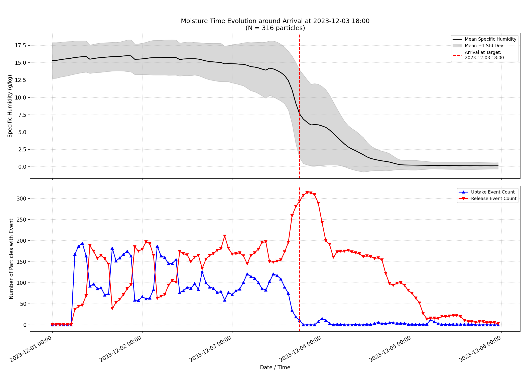Figure 15: Example Time Evolution Plot (Multi-Step Focus).

5.6. Animation Generation (animations.py)

This module creates animated sequences from frames generated by plotting_2d.py and plotting_3d.py.

5.6.1. Main Function: create_all_animations

This function orchestrates the generation of hourly snapshot frames and compiles them into animations.

• Purpose: To generate 2D and 3D animations of hourly particle snapshots.
• Methodology:
  1. Calculates global normalization ranges for q (g/kg) and T (K) across all animation frames to ensure consistent color scales. Uses percentiles (e.g., 0.5th and 99.5th) for robustness.
  2. Determines fixed plot extents for 2D animations (FIXED_PLOT_EXTENT_2D or dynamic) and 3D animations (FIXED_PLOT_LONLAT_EXTENT_3D, FIXED_PLOT_PRESSURE_EXTENT_3D or dynamic).
  3. Generates static colorbar images for q and T using _generate_static_colorbar.
  4. For each hour from ANIMATION_FRAME_START_HOUR to ANIMATION_FRAME_END_HOUR:
     • Calls plotting_2d.generate_2d_snapshot_frame to create 2D frames (one for q, one for T). Particles are colored by the respective variable.
     • Calls plotting_3d.generate_3d_snapshot_frame to create 3D frames (one for q, one for T). Particles are colored by the respective variable.
     • Frames are saved to subdirectories under PLOTS_OUTPUT_DIR/animation_frames/.
  5. Compiles the generated 2D and 3D frames for q and T into separate GIF and MP4 animations using imageio via _compile_animation_files. Animation speed is controlled by ANIMATION_FPS.
• Output: GIF and MP4 animation files, and static colorbar PNGs, saved in PLOTS_OUTPUT_DIR/animations_output/.

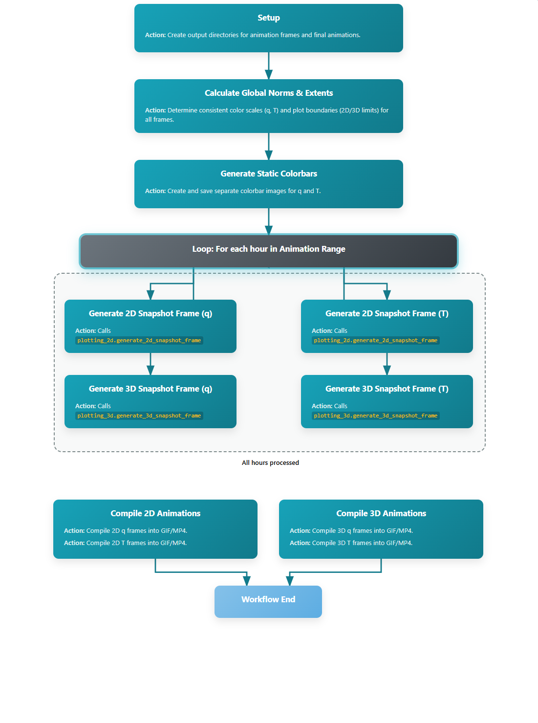Figure 16: Flowchart of Animation Generation Process - Animation Generation Workflow.

Figure 17: Sample of a 3D Moisture Animation.

5.7. Moisture Tracks Analysis (MoistureTracks.py)

This module focuses on particles that contribute moisture to the target area through release events. It analyzes their trajectories and spatial distribution of moisture release.

5.7.1. Main Function: run_moisture_tracks_analysis

• Purpose: Identifies particles releasing moisture in the target area and generates analyses of their behavior.
• Methodology:
  1. Filters master_df for "Release" events in the target area to identify moisture-releasing particles.
  2. Generates cumulative trajectory plots for all releasing particles, colored by pressure or release amount.
  3. Creates hourly trajectory plots for particles arriving at target at specific hours.
  4. Computes and plots net moisture flux (uptake - release) aggregated on a grid.
  5. Grids spatial moisture contribution, aggregating release amounts per grid cell and generating a heatmap/map with CSV export.
  6. Plots time evolution of specific humidity and change for releasing particles.
  7. Plots total specific humidity in target over time.
  8. Generates hourly Excel files with specific humidity details.
• Output: Trajectory maps, net flux maps, contribution heatmaps, time evolution plots, Excel data files, all saved in MOISTURE_TRACKS_OUTPUT_DIR.

5. Configuration (config.py)

The config.py file is central to the entire workflow. It allows users to customize nearly every aspect of the analysis without modifying the core processing scripts. Key sections include:

• Core Simulation & Data Paths (e.g., BASE_OUTPUT_DIR, AUGMENTED_PARTICLE_DATA_DIR)
• Event Definition & Particle Selection (e.g., SIMULATION_START_DATETIME, TARGET_LAT_CENTER, RELEVANT_PARTICLE_TARGET_ARRIVAL_STEPS)
• Detailed Analysis Configuration (e.g., ANALYSIS_START_HOUR, DQ_THRESHOLD_KG_PER_KG, CHANGE_WINDOW_HOURS)
• Plotting & Animation Configuration (e.g., FIXED_PLOT_EXTENT_2D, ANIMATION_FPS, Colormaps like CMAP_SPECIFIC_HUMIDITY)
• Tracks Analysis Specific Settings (e.g., TRACKS_TARGET_STEPS, TRACKS_PLOT_EXTENT_2D)
• Parallel Processing (NUM_WORKERS)
• Output Subdirectory Definitions (e.g., INDIVIDUAL_TRAJ_PLOTS_SUBDIR)

Careful adjustment of these parameters is crucial for obtaining meaningful results tailored to specific research questions or datasets.

6. Expected Outputs

The analysis pipeline generates a variety of outputs, organized into subdirectories within the BASE_OUTPUT_DIR specified in config.py. These include:

• Processed Data (under 1_processed_data/):
  • relevant_particle_ids_for_analysis.csv: List of particle IDs selected for detailed analysis.
  • filtered_hourly_data/: Hourly CSVs containing only data for relevant particles.
  • analyzed_particle_histories/: CSVs for each relevant particle with calculated dq/dt, dT/dt, event types, etc.
  • tracks_analysis_output/data_from_master/: CSVs from tracks analysis (initial/final states).
  • moisture_tracks_output/: Data and Excel files from moisture tracks analysis.
• Plots & Animations (under 2_plots_and_animations/):
  • aggregate_maps/: Static 2D aggregate maps (PNG).
  • individual_trajectories/: Static 2D and 3D individual trajectory plots (PNG).
  • statistical_distributions/, target_area_analysis/, time_evolution/: Various statistical plots (PNG).
  • tracks_analysis_output/plots_from_master/: Plots from tracks analysis (PNG).
  • animation_frames/: Individual frames for animations (PNG).
  • animations_output/: Compiled 2D and 3D animations (GIF, MP4) and static colorbars (PNG).

BASE_OUTPUT_DIR/
├── 1_processed_data/
│   ├── filtered_hourly_data/
│   └── analyzed_particle_histories/
└── 2_plots_and_animations/
    ├── tracks_analysis_output/
    │   ├── data_from_master/
    │   └── plots_from_master/
    │       └── change_along_trajectory/
    ├── individual_trajectories/
    │   ├── Moisture/
    │   ├── Temperature/
    │   └── 3D/
    │       ├── Moisture/
    │       └── Temperature/
    ├── aggregate_maps_moisture/
    ├── aggregate_maps_temp/
    ├── animation_frames_2d/
    │   ├── specific_humidity/
    │   └── temperature/
    ├── animation_frames_3d/
    │   ├── specific_humidity/
    │   └── temperature/
    ├── animations_output/
    ├── statistical_distributions_moisture/
    │   ├── profile_change_vs_mean_p_6hr/
    │   └── profile_change_vs_mean_p_1hr/
    ├── statistical_distributions_temp/
    │   ├── profile_change_vs_mean_p_6hr/
    │   └── profile_change_vs_mean_p_1hr/
    ├── target_area_analysis/
    └── time_evolution/

Authors

Manish Shukla - Postdoctoral student, Indian Institute of Technology Hyderabad (manishshukla01@live.com)

R. Maheshwaran - Assistant Professor, Indian Institute of Technology Hyderabad

7. Future Enhancements / Considerations

• Integration of more sophisticated statistical analysis methods (e.g., clustering).
• Interactive plotting capabilities (e.g., using Bokeh or Plotly).
• More detailed source-receptor relationship analysis.
• Optimization of data loading and processing for very large datasets.